pyPESTO: Getting started

This notebook takes you through the first steps to get started with pyPESTO.

pyPESTO is a python package for parameter inference, offering a unified interface to various optimization and sampling methods. pyPESTO is highly modular and customizable, e.g., with respect to objective function definition and employed inference algorithms.

import logging

import amici.sim.sundials as asd
import matplotlib as mpl
import numpy as np

import pypesto.optimize as optimize
import pypesto.petab
import pypesto.visualize as visualize

np.random.seed(1)

# increase image resolution
mpl.rcParams["figure.dpi"] = 300

1. Objective Definition

pyPESTO allows the definition of custom objectives and offers support for objectives defined in the PEtab format.

Custom Objective Definition

You can define an objective via a python function. Also providing an analytical gradient (and potentially also a Hessian) improves the performance of Gradient/Hessian-based optimizers. When accessing parameter uncertainties via profile-likelihoods/sampling, pyPESTO interprets the objective function as the negative-log-likelihood/negative-log-posterior. A more in-depth construction of a custom objective function can be found in a designated example notebook.

# define objective function
def f(x: np.ndarray) -> np.ndarray:
    return x[0] ** 2 + x[1] ** 2


# define gradient
def grad(x: np.ndarray) -> np.ndarray:
    return 2 * x


# define objective
custom_objective = pypesto.Objective(fun=f, grad=grad)

Define lower and upper parameter bounds and create an optimization problem.

# define optimization bounds
lb = np.array([-10, -10])
ub = np.array([10, 10])

# create problem
custom_problem = pypesto.Problem(objective=custom_objective, lb=lb, ub=ub)

Now choose an optimizer to perform the optimization. minimize uses multi-start optimization, meaning that the optimization is run n_start times from different initial values, in case the problem contains multiple local optima (which of course is not the case for this toy problem).

# choose optimizer
optimizer = optimize.ScipyOptimizer()

# do the optimization
result_custom_problem = optimize.minimize(
    problem=custom_problem, optimizer=optimizer, n_starts=10
)

result_custom_problem.optimize_result now stores a list, that contains the results and metadata of the individual optimizer runs (ordered by function value).

# E.g., The best model fit was obtained by the following optimization run:
result_custom_problem.optimize_result.list[0]

{'id': '2',
 'x': array([0., 0.]),
 'fval': np.float64(0.0),
 'grad': array([0., 0.]),
 'hess': None,
 'res': None,
 'sres': None,
 'n_fval': 4,
 'n_grad': 4,
 'n_hess': 0,
 'n_res': 0,
 'n_sres': 0,
 'x0': array([-7.06488218, -8.1532281 ]),
 'fval0': np.float64(116.38768879499594),
 'history': <pypesto.history.base.CountHistory at 0x762d61303f10>,
 'exitflag': 0,
 'time': 0.0011506080627441406,
 'message': 'CONVERGENCE: NORM OF PROJECTED GRADIENT <= PGTOL',
 'optimizer': "<ScipyOptimizer method=L-BFGS-B options={'maxfun': 1000}>",
 'free_indices': array([0, 1]),
 'inner_parameters': None,
 'spline_knots': None}

# Objective function values of the different optimizer runs:
result_custom_problem.optimize_result.get_for_key("fval")

[np.float64(0.0),
 np.float64(0.0),
 np.float64(0.0),
 np.float64(0.0),
 np.float64(0.0),
 np.float64(0.0),
 np.float64(1.504632769052528e-36),
 np.float64(3.056285312137946e-36),
 np.float64(3.76158192263132e-36),
 np.float64(3.76158192263132e-36)]

Problem Definition via PEtab

Background on PEtab

PyPESTO supports the PEtab standard. PEtab is a data format for specifying parameter estimation problems in systems biology.

A PEtab problem consist of an SBML file, defining the model topology and a set of .tsv files, defining experimental conditions, observables, measurements and parameters (and their optimization bounds, scale, priors…). All files that make up a PEtab problem can be structured in a .yaml file. The pypesto.Objective coming from a PEtab problem corresponds to the negative-log-likelihood/negative-log-posterior distribution of the parameters.

For more details on PEtab, the interested reader is referred to PEtab’s format definition, for examples, the reader is referred to the PEtab benchmark collection. The Model from Böhm et al. JProteomRes 2014 is part of the benchmark collection and will be used as the running example throughout this notebook.

PyPESTO provides an interface to the model simulation tool AMICI for the simulation of Ordinary Differential Equation (ODE) models specified in the SBML format.

Basic Model Import and Optimization

The first step is to import a PEtab problem and create a pypesto.problem object:

%%capture
# directory of the PEtab problem
petab_yaml = "./conversion_reaction/conversion_reaction.yaml"

importer = pypesto.petab.PetabImporter.from_yaml(petab_yaml)
problem = importer.create_problem(verbose=False)

Compiling amici model to folder /home/docs/checkouts/readthedocs.org/user_builds/pypesto/checkouts/1652/doc/example/amici_models/1.0.0/conversion_reaction_0.

petab_yaml

'./conversion_reaction/conversion_reaction.yaml'

Next, we choose an optimizer to perform the multi start optimization.

%%time
%%capture

# choose optimizer
optimizer = optimize.ScipyOptimizer()

# do the optimization
result = optimize.minimize(problem=problem, optimizer=optimizer, n_starts=5)

CPU times: user 409 ms, sys: 11.5 ms, total: 420 ms
Wall time: 224 ms

result.optimize_result contains a list with the ordered optimization results.

# E.g., best model fit was obtained by the following optimization run:
result.optimize_result.list[0]

{'id': '3',
 'x': array([-0.25416784, -0.60834099]),
 'fval': -25.356201814389237,
 'grad': array([ 5.90098791e-06, -4.77905881e-06]),
 'hess': None,
 'res': None,
 'sres': None,
 'n_fval': 46,
 'n_grad': 46,
 'n_hess': 0,
 'n_res': 0,
 'n_sres': 0,
 'x0': array([ 4.42839188, -7.60243554]),
 'fval0': 3275.6428996850577,
 'history': <pypesto.history.base.CountHistory at 0x762d6186e810>,
 'exitflag': 0,
 'time': 0.10239434242248535,
 'message': 'CONVERGENCE: NORM OF PROJECTED GRADIENT <= PGTOL',
 'optimizer': "<ScipyOptimizer method=L-BFGS-B options={'maxfun': 1000}>",
 'free_indices': array([0, 1]),
 'inner_parameters': None,
 'spline_knots': None}

# Objective function values of the different optimizer runs:
result.optimize_result.get_for_key("fval")

[-25.356201814389237,
 49.9096545687522,
 132.61011287146414,
 132.61011287146414,
 3275.7137352431205]

2. Optimizer Choice

PyPESTO provides a unified interface to a variety of optimizers of different types. Examples are:

• All scipy optimizer (optimize.ScipyOptimizer(method=<method_name>))

  • function-value or least-squares-based optimizers

  • gradient or hessian-based optimizers

• IpOpt (optimize.IpoptOptimizer())

  • Interior point method

• Dlib (optimize.DlibOptimizer(options={'maxiter': <max. number of iterations>}))

  • Global optimizer

  • Gradient-free

• FIDES (optimize.FidesOptimizer())

  • Interior Trust Region optimizer

• Particle Swarm (optimize.PyswarmsOptimizer())

  • Particle swarm algorithm

  • Gradient-free

• CMA-ES (optimize.CmaOptimizer())

  • Covariance Matrix Adaptation Evolution Strategy

  • Evolutionary Algorithm

optimizer_scipy_lbfgsb = optimize.ScipyOptimizer(method="L-BFGS-B")
optimizer_scipy_powell = optimize.ScipyOptimizer(method="Powell")

optimizer_fides = optimize.FidesOptimizer(verbose=logging.ERROR)
optimizer_pyswarms = optimize.PyswarmsOptimizer(par_popsize=10)

The following performs 10 multi-start runs with different optimizers in order to compare their performance. For a faster execution of this notebook, we run only 10 starts. In application, one would use many more optimization starts: around 100-1000 in most cases.

Note: Some of those optimizers need to be installed separately for this section to run (e.g., via pip install pypesto[fides,pyswarms]). Furthermore, the computation time is in the order of minutes, so you might want to skip the execution and jump to the section on large scale models.

%%time
%%capture --no-display
n_starts = 10

# Due to run time we already use parallelization.
# This will be introduced in more detail later.
engine = pypesto.engine.MultiProcessEngine()

# Scipy: L-BFGS-B
result_lbfgsb = optimize.minimize(
    problem=problem,
    optimizer=optimizer_scipy_lbfgsb,
    engine=engine,
    n_starts=n_starts,
)

# Scipy: Powell
result_powell = optimize.minimize(
    problem=problem,
    optimizer=optimizer_scipy_powell,
    engine=engine,
    n_starts=n_starts,
)

# Fides
result_fides = optimize.minimize(
    problem=problem,
    optimizer=optimizer_fides,
    engine=engine,
    n_starts=n_starts,
)

# PySwarms
result_pyswarms = optimize.minimize(
    problem=problem,
    optimizer=optimizer_pyswarms,
    engine=engine,
    n_starts=1,  # Global optimizers are usually run once. The number of particles (par_popsize) is usually the parameter that is adapted.
)

Engine will use up to 2 processes (= CPU count).
The pyswarms optimizer does not support x0.
The pyswarms optimizer does not support x0.

CPU times: user 110 ms, sys: 119 ms, total: 229 ms
Wall time: 7.8 s

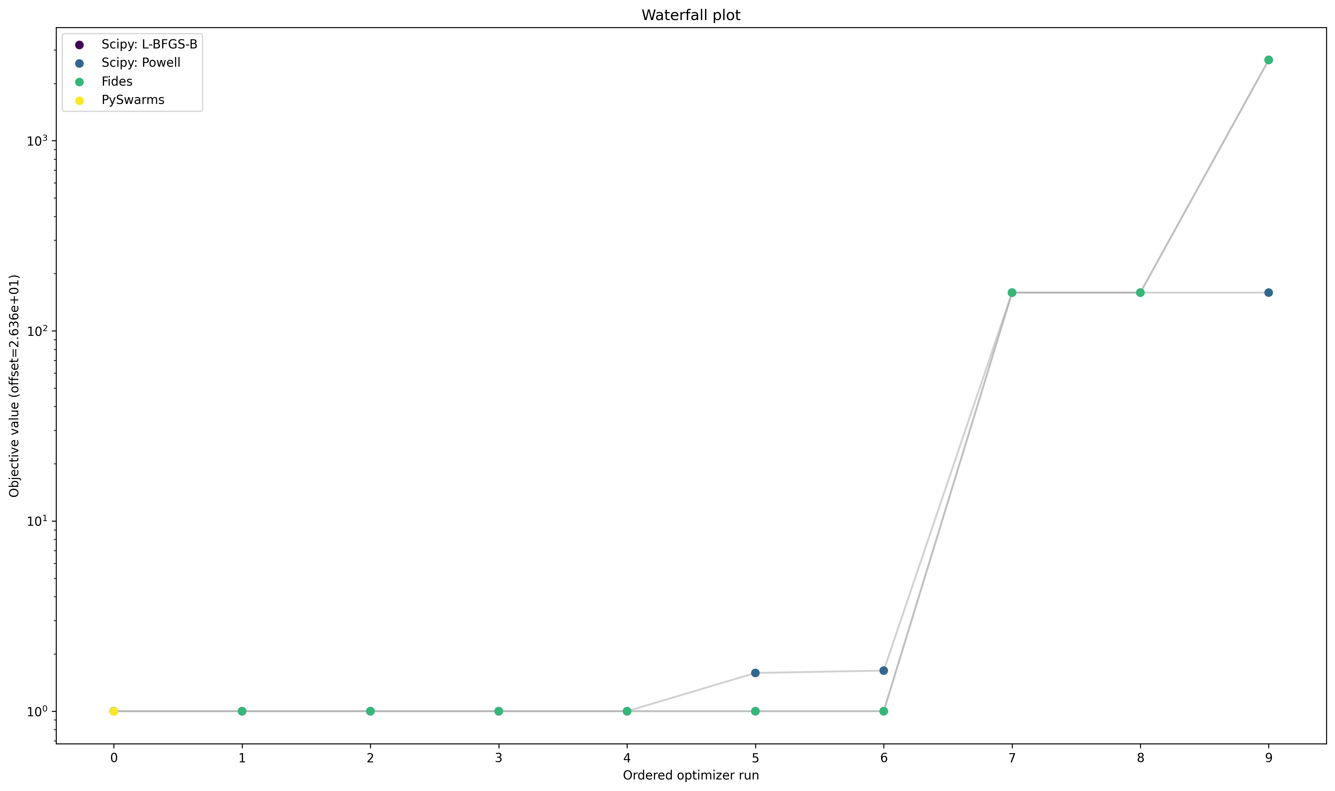
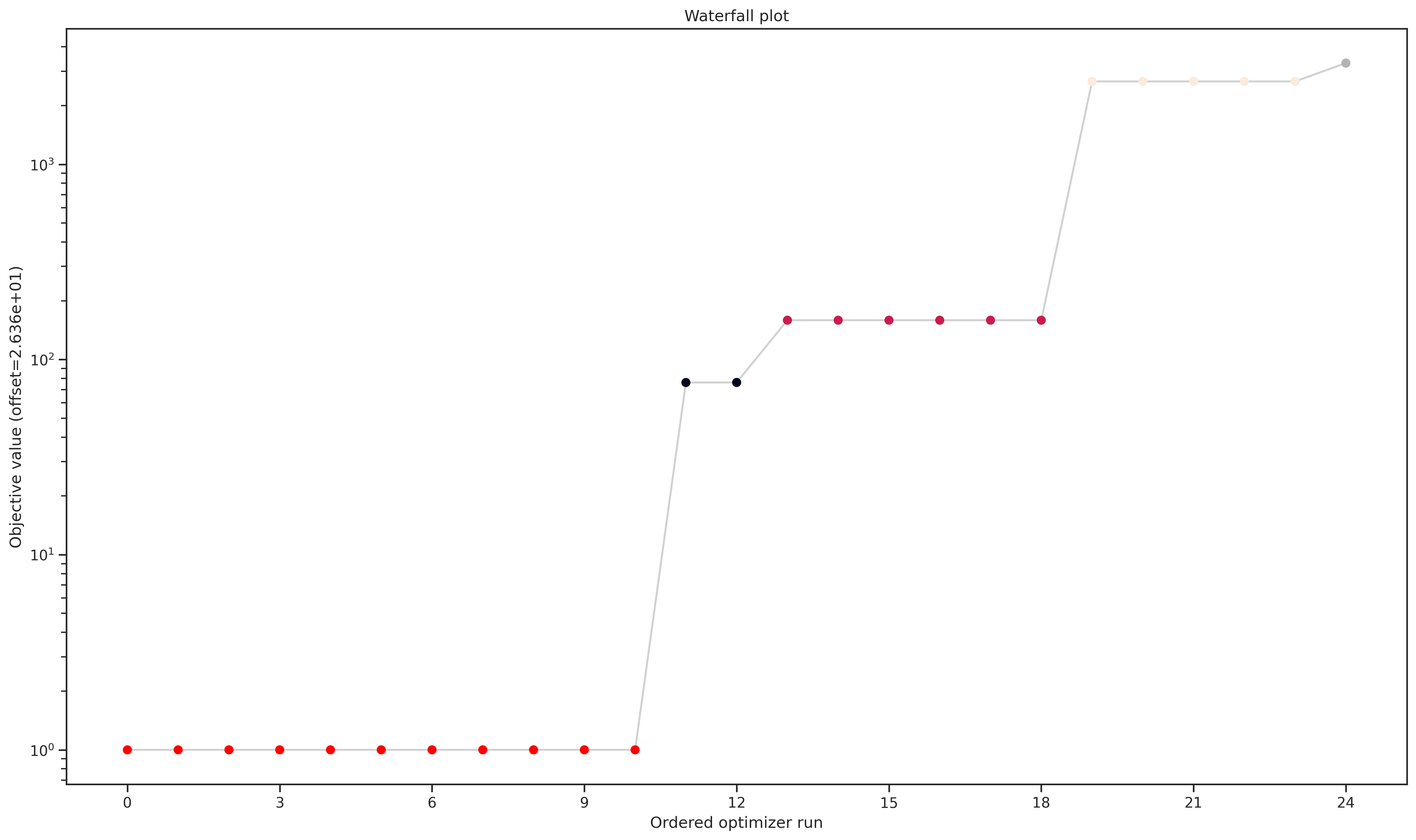
Optimizer Convergence

A common visualization of optimizer convergence are waterfall plots. Waterfall plots show the (ordered) results of the individual optimization runs. In general, we hope to obtain clearly visible plateaus, as they indicate optimizer convergence to local minima.

optimizer_results = [
    result_lbfgsb,
    result_powell,
    result_fides,
    result_pyswarms,
]
optimizer_names = ["Scipy: L-BFGS-B", "Scipy: Powell", "Fides", "PySwarms"]

pypesto.visualize.waterfall(optimizer_results, legends=optimizer_names);

Optimizer run time

Optimizer run time vastly differs among the different optimizers, as can be seen below:

print("Average Run time per start:")
print("-------------------")

for optimizer_name, optimizer_result in zip(
    optimizer_names, optimizer_results, strict=True
):
    t = np.sum(optimizer_result.optimize_result.get_for_key("time")) / n_starts
    print(f"{optimizer_name}: {t:f} s")

Average Run time per start:
-------------------
Scipy: L-BFGS-B: 0.187293 s
Scipy: Powell: 0.147819 s
Fides: 0.065401 s
PySwarms: 0.479350 s

3. Fitting of large scale models

When fitting large scale models (i.e. with >100 parameters and accordingly also more data), two important issues are efficient gradient computation and parallelization.

Efficient gradient computation

As seen in the example above and as can be confirmed from own experience: If fast and reliable gradients can be provided, gradient-based optimizers are favourable with respect to optimizer convergence and run time.

It has been shown that adjoint sensitivity analysis is a fast and reliable method to compute gradients for large scale models, since their run time is (asymptotically) independent of the number of parameters (Fröhlich et al. PlosCB 2017).

(Figure from Fröhlich et al. PlosCB 2017) Adjoint sensitivities are implemented in AMICI.

# Set gradient computation method to adjoint
problem.objective.amici_solver.set_sensitivity_method(
    asd.SensitivityMethod.adjoint
)

Parallelization

Multi-start optimization can easily be parallelized by using engines.

%%time
%%capture

# Parallelize
engine = pypesto.engine.MultiProcessEngine()

# Optimize
result = optimize.minimize(
    problem=problem,
    optimizer=optimizer_scipy_lbfgsb,
    engine=engine,
    n_starts=25,
)

Engine will use up to 2 processes (= CPU count).

CPU times: user 68.7 ms, sys: 51.5 ms, total: 120 ms
Wall time: 5.66 s

4. Uncertainty quantification

PyPESTO focuses on two approaches to assess parameter uncertainties:

• Profile likelihoods

• Sampling

Profile Likelihoods

Profile likelihoods compute confidence intervals via a likelihood ratio test. Profile likelihoods perform a maximum-projection of the likelihood function on the parameter of interest. The likelihood ratio test then gives a cut-off criterion via the \(\chi^2_1\) distribution.

In pyPESTO, the maximum projection is solved as a maximization problem and can be obtained via

%%time
%%capture

import scipy as sp

import pypesto.profile as profile

options = profile.ProfileOptions(
    ratio_min=np.exp(-sp.stats.chi2.ppf(0.99, 1) / 2)
)
result = profile.parameter_profile(
    problem=problem,
    result=result,
    optimizer=optimizer_scipy_lbfgsb,
    profile_index=[0, 1],
    profile_options=options,
)

CPU times: user 11.1 s, sys: 103 ms, total: 11.2 s
Wall time: 7.56 s

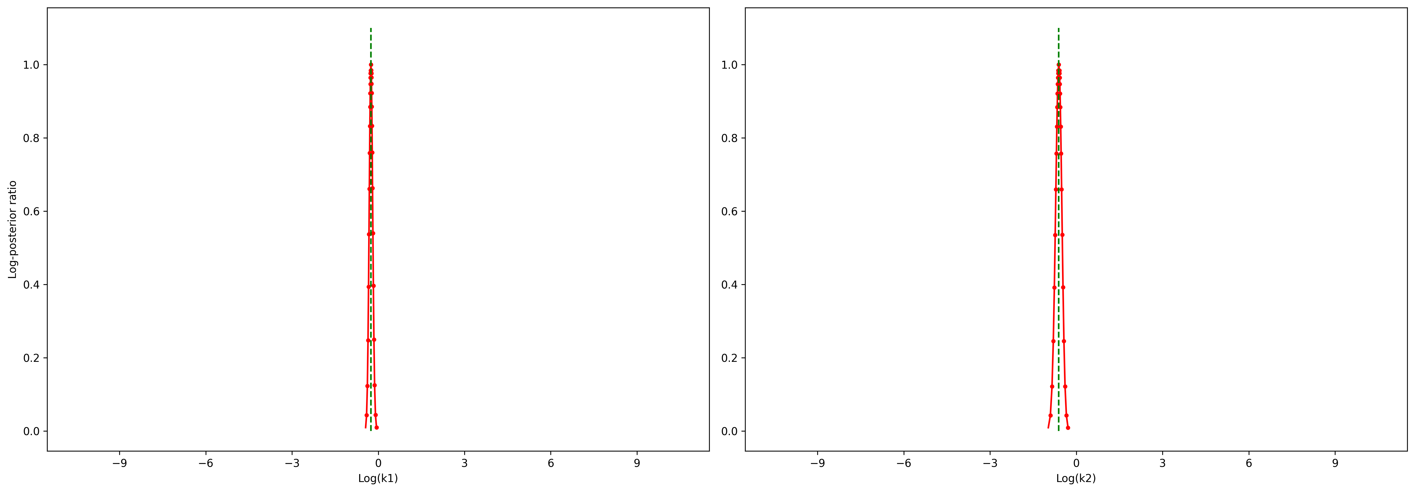
The maximum projections can now be inspected via:

problem.x_scales

['log', 'log']

# adapt x_labels.
x_labels = [f"Log({name})" for name in problem.x_names]

ax = visualize.profiles(result, x_labels=x_labels, show_bounds=True)
# visualize optimal parameter values
ax[0].plot(
    [result_fides.optimize_result.x[0][0]] * 2,
    [0, 1.1],
    linestyle="--",
    color="g",
)
ax[1].plot(
    [result_fides.optimize_result.x[0][1]] * 2,
    [0, 1.1],
    linestyle="--",
    color="g",
)

[<matplotlib.lines.Line2D at 0x762d60776090>]

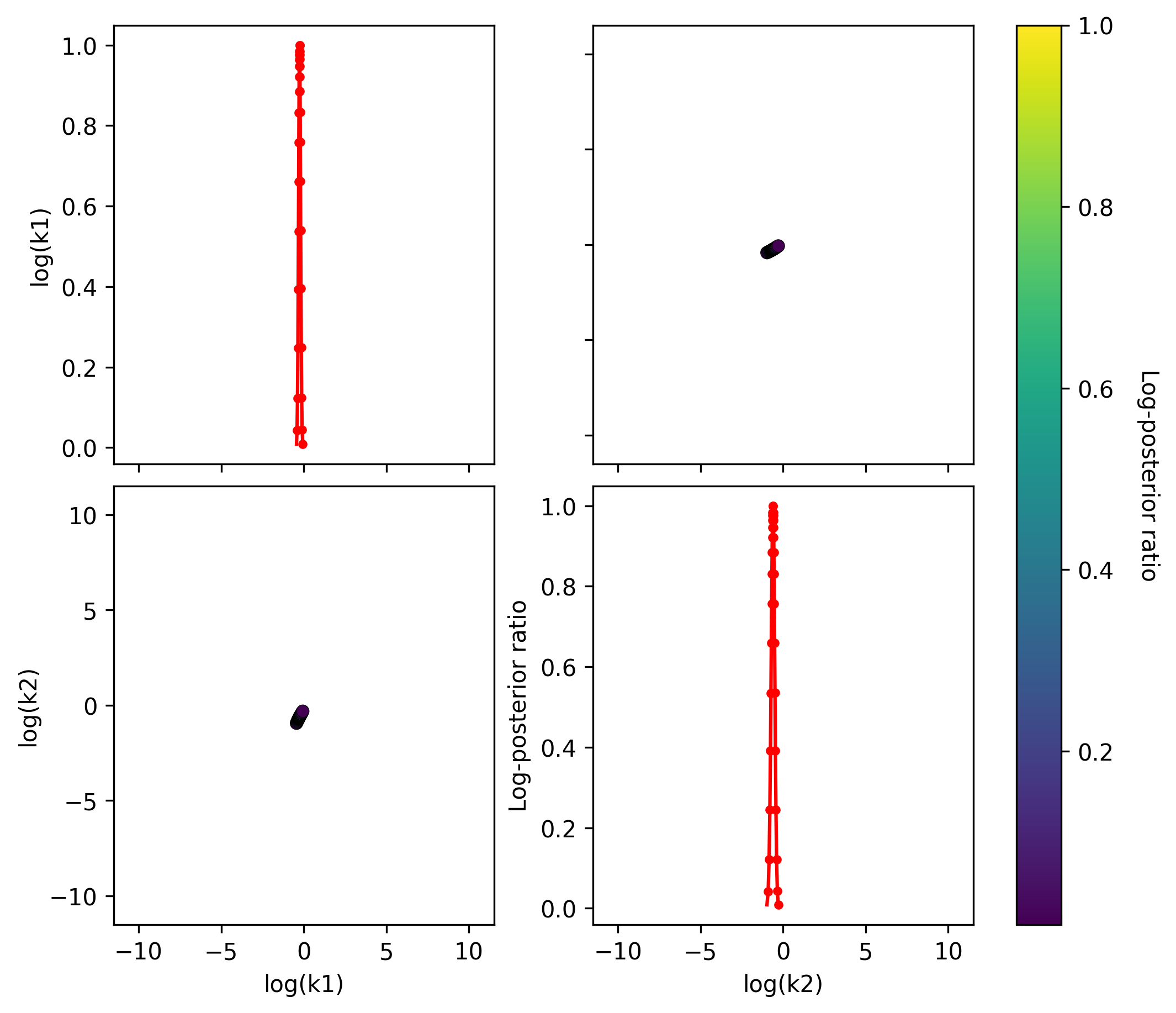
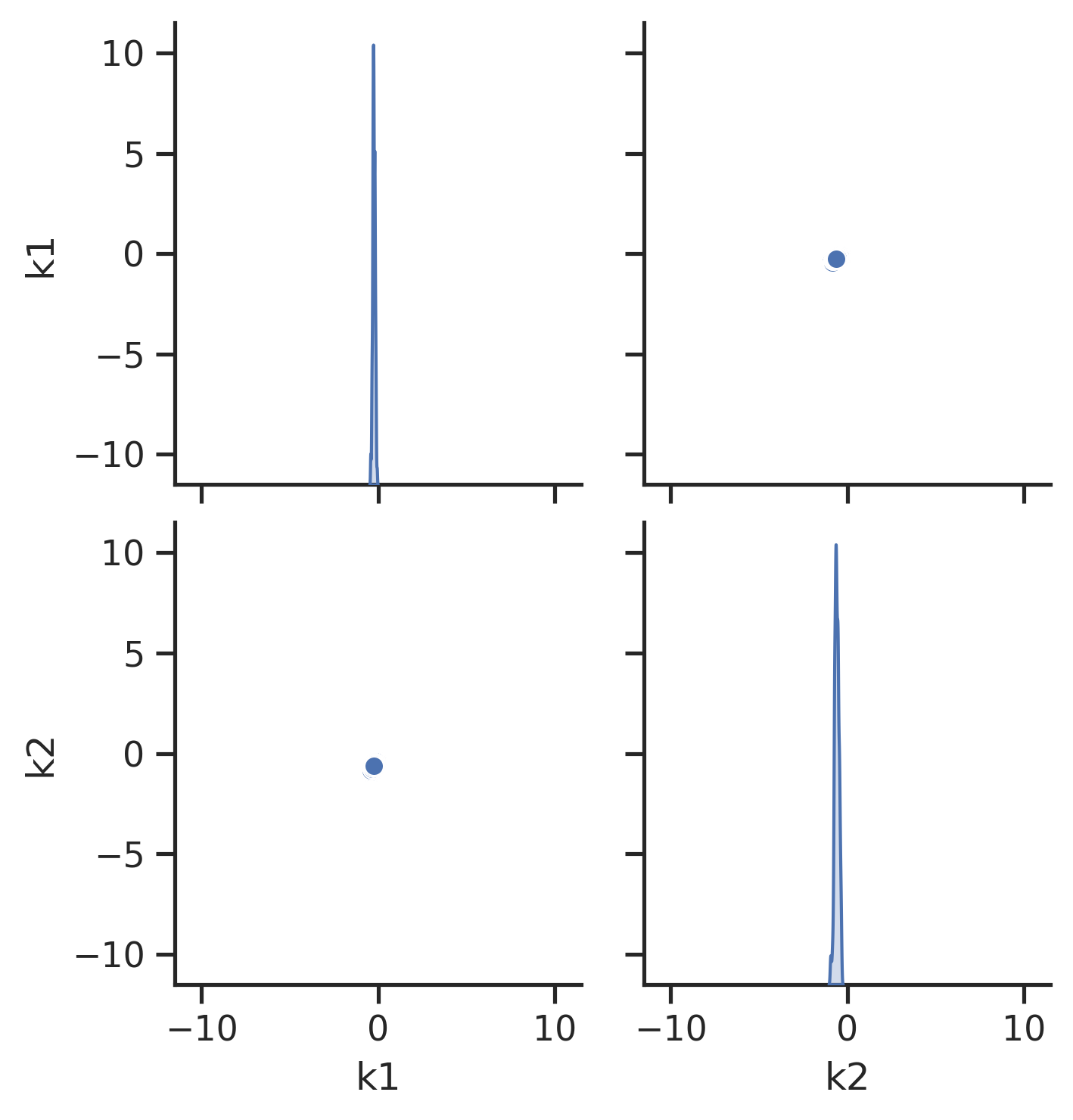
The 2D profile visualization shows joint parameter paths across all profile pairs. Diagonal plots show 1D profiles (likelihood ratio vs. parameter value). Off-diagonal plots show how each non-profiled parameter moves while another is profiled, with color indicating the likelihood ratio.

fig, axes = pypesto.visualize.visualize_2d_profile(result)

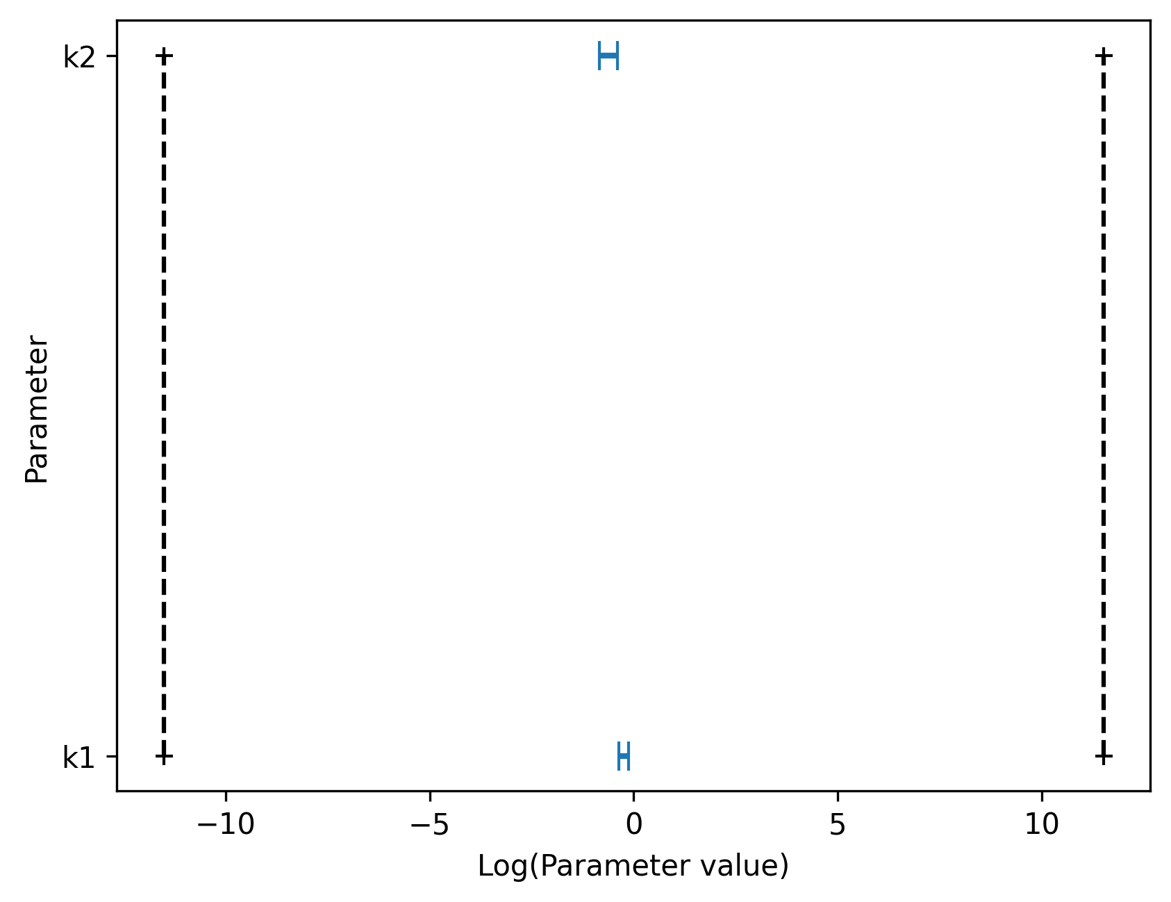
Furthermore, pyPESTO allows to visualize approximate confidence intervals directly via profile_cis. Confidence intervals are computed by finding parameter values for which the log posterior ratio is above the approximate threshold assuming a \(\chi^2\) distribution of the likelihood test statistic. The plot shows that both model parameters are identifiable, since the confidence regions are finite and do not span the whole estimation space (from lower to upper estimation boundary).

ax = pypesto.visualize.profile_cis(
    result, confidence_level=0.95, show_bounds=True
)

ax.set_xlabel("Log(Parameter value)");

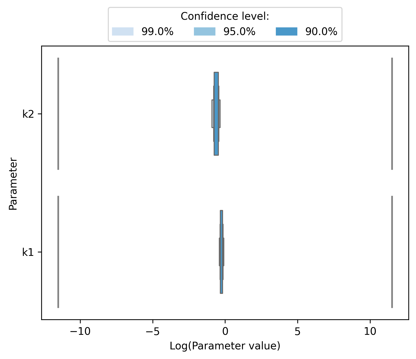
Parameter profiles need to be computed until the likelihood ratio is small enough to compute confidence intervals with the selected confidence level (see ratio_min attribute of ProfileOptions). It is also possible to visualize nested confidence intervals corresponding to different confidence levels.

ax = pypesto.visualize.profile_nested_cis(
    result, confidence_levels=[0.99, 0.95, 0.9]
)

ax.set_xlabel("Log(Parameter value)");

Sampling

In pyPESTO, sampling from the posterior distribution can be performed as

import pypesto.sample as sample

n_samples = 1000

sampler = sample.AdaptiveMetropolisSampler()

result = sample.sample(
    problem, n_samples=n_samples, sampler=sampler, result=result
)

Elapsed time: 0.6420578219999982

Sampling results are stored in result.sample_result and can be accessed e.g., via

result.sample_result["trace_x"]

array([[[-0.25416727, -0.60833968],
        [-0.25416727, -0.60833968],
        [-0.25416727, -0.60833968],
        ...,
        [-0.26079315, -0.6205545 ],
        [-0.26079315, -0.6205545 ],
        [-0.26079315, -0.6205545 ]]], shape=(1, 1001, 2))

Sampling Diagnostics

Geweke’s test assesses convergence of a sampling run and computes the burn-in of a sampling result. The effective sample size indicates the strength of the correlation between different samples.

sample.geweke_test(result=result)
result.sample_result["burn_in"]

Geweke burn-in index: 0

np.int64(0)

sample.effective_sample_size(result=result)
result.sample_result["effective_sample_size"]

Estimated chain autocorrelation: 7.526115594067884
Estimated effective sample size: 117.40399117934246

np.float64(117.40399117934246)

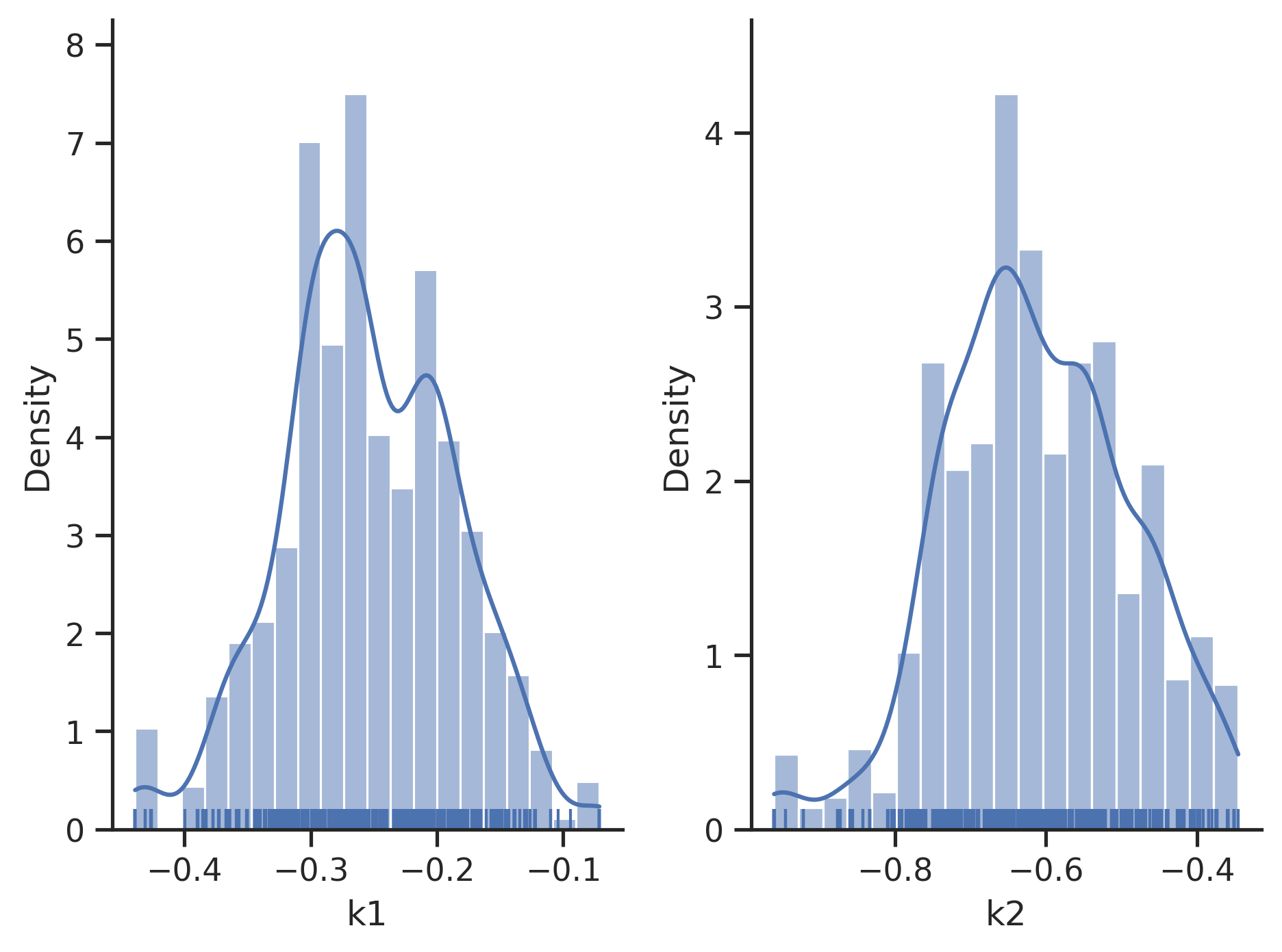
Visualization of Sampling Results

# scatter plots
visualize.sampling_scatter(result)

# marginals
visualize.sampling_1d_marginals(result);

Sampler Choice:

Similarly to parameter optimization, pyPESTO provides a unified interface to several sampler/sampling toolboxes, as well as own implementations of samplers:

• Adaptive Metropolis: pypesto.sample.AdaptiveMetropolisSampler()

• Parallel tempering: pypesto.sample.ParallelTemperingSampler()

• Adaptive parallel tempering: pypesto.sample.AdaptiveParallelTemperingSampler()

• Interface to pymc 🔗 via pypesto.sample.PymcSampler()

5. Storage

You can store and load the results of an analysis via the pypesto.store module to a .hdf5 file.

Store result

import tempfile

import pypesto.store as store

# create a temporary file, for demonstration purpose
f_tmp = tempfile.NamedTemporaryFile(suffix=".hdf5", delete=False)
result_file_name = f_tmp.name

# store the result
store.write_result(result, result_file_name)
f_tmp.close()

Load result file

You can re-load a result, e.g. for visualizations:

# read result
result_loaded = store.read_result(result_file_name)

# e.g. do some visualisation
visualize.waterfall(result_loaded);

Software Development Standards:

PyPESTO is developed with the following standards:

• Open source, code on GitHub.

• Pip installable via: pip install pypesto.

• Documentation as RTD and example jupyter notebooks are available.

• Has continuous integration & extensive automated testing.

• Code reviews before merging into the develop/main branch.

• Currently, 5–10 people are using, extending and (most importantly) maintaining pyPESTO in their “daily business”.

Further topics

Further features are available, among them:

• Model Selection

• Hierarchical Optimization of scaling/noise parameters

• Categorical Data