Bayes Factor Tutorial

Bayes factors are a key concept in Bayesian model comparison, allowing us to compare the relative likelihood of different models given the data. They are computed using the marginal likelihoods (or evidence) of the models. This tutorial will cover various methods for computing marginal likelihoods.

You find an introduction and extensive review here: Llorente et al. (2023).

Marginal Likelihood

The marginal likelihood (or evidence) of a model \(\mathcal{M}\) given data \(\mathcal{D}\) is defined as:

\[P(\mathcal{D} \mid \mathcal{M}) = \int P(\mathcal{D} \mid \theta, \mathcal{M}) P(\theta \mid \mathcal{M}) \, d\theta\]

where \(\theta\) are the parameters of the model. This integral averages the likelihood over the prior distribution of the parameters, providing a measure of how well the model explains the data, considering all possible parameter values.

Bayes Factor

The Bayes factor comparing two models \(\mathcal{M}_1\) and \(\mathcal{M}_2\) given data \(\mathcal{D}\) is the ratio of their marginal likelihoods:

\[\operatorname{BF}_{12} = \frac{P(\mathcal{D} \mid \mathcal{M}_1)}{P(\mathcal{D} \mid \mathcal{M}_2)}\]

A \(\operatorname{BF}_{12} > 1\) indicates that the data favors model \(\mathcal{M}_1\) over model \(\mathcal{M}_2\), while \(\operatorname{BF}_{12} < 1\) indicates the opposite.

Jeffreys (1961) suggested interpreting Bayes factors in half-units on the log10 scale (this was further simplified in Kass and Raftery (1995)):

Not worth more than a bare mention: \(0 < \log_{10} \operatorname{BF}_{12} \leq 0.5\)
Substantial: \(0.5 < \log_{10}\operatorname{BF}_{12} \leq 1\)
Strong: \(1 < \log_{10}\operatorname{BF}_{12} \leq 2\)
Decisive: \(2 < \log_{10}\operatorname{BF}_{12}\)

Example

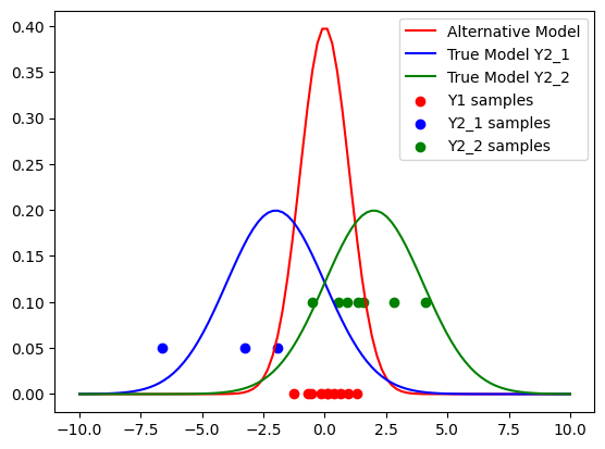
To illustrate different methods to compute marginal likelihoods, we introduce two toy models, for which we can compute the marginal likelihoods analytically:

Mixture of Two Gaussians (True Data Generator): Composed of two Gaussian distributions, \(\mathcal{N}(\mu_1, \sigma_1^2)\) and \(\mathcal{N}(\mu_2, \sigma_2^2)\), with mixing coefficient \(\pi=0.7\).
Single Gaussian (Alternative Model): A single Gaussian distribution, \(\mathcal{N}(\mu, \sigma^2)\).

We sample synthetic data from the first model and create pypesto problems for both models with the same data. The free parameters are the means of both models. For this example, we assume that the standard deviation is known and fixed to the true value. As priors, we assume normal distributions.

[1]:

from functools import partial

import matplotlib.pyplot as plt
import numpy as np
from scipy import stats
from scipy.special import logsumexp

from pypesto import optimize, sample, variational, visualize
from pypesto.C import LIN, NORMAL
from pypesto.objective import (
    AggregatedObjective,
    NegLogParameterPriors,
    Objective,
    get_parameter_prior_dict,
)
from pypesto.problem import Problem

# For testing purposes. Remove if not running the exact example.
np.random.seed(42)

[2]:

# model hyperparameters
N = 10
N2_1 = 3
N2_2 = N - N2_1
sigma2 = 2.0
true_params = np.array([-2.0, 2.0])

rng = np.random.default_rng(seed=0)
# Alternative Model
Y1 = rng.normal(loc=0.0, scale=1.0, size=N)

# True Model
Y2_1 = rng.normal(loc=true_params[0], scale=sigma2, size=N2_1)
Y2_2 = rng.normal(loc=true_params[1], scale=sigma2, size=N2_2)
Y2 = np.concatenate([Y2_1, Y2_2])
mixture_data, sigma = Y2, sigma2
n_obs = len(mixture_data)

# plot the alternative model distribution as a normal distribution
plt.figure()
x = np.linspace(-10, 10, 100)
plt.plot(
    x,
    stats.norm.pdf(x, loc=0.0, scale=1.0),
    label="Alternative Model",
    color="red",
)
plt.plot(
    x,
    stats.norm.pdf(x, loc=true_params[0], scale=sigma2),
    label="True Model Y2_1",
    color="blue",
)
plt.plot(
    x,
    stats.norm.pdf(x, loc=true_params[1], scale=sigma2),
    label="True Model Y2_2",
    color="green",
)


# Plot the data of the alternative and true model as dots on the x-axis for each model
plt.scatter(Y1, np.zeros_like(Y1), label="Y1 samples", color="red")
plt.scatter(Y2_1, np.full(len(Y2_1), 0.05), label="Y2_1 samples", color="blue")
plt.scatter(Y2_2, np.full(len(Y2_2), 0.1), label="Y2_2 samples", color="green")
plt.legend()
plt.show()

../_images/example_model_evidence_and_bayes_factors_5_0.png

[3]:

# evidence
def log_evidence_alt(data: np.ndarray, std: float):
    n = int(data.size)
    y_sum = np.sum(data)
    y_sq_sum = np.sum(data**2)

    term1 = 1 / (np.sqrt(2 * np.pi) * std)
    log_term2 = -0.5 * np.log(n + 1)
    inside_exp = -0.5 / (std**2) * (y_sq_sum - (y_sum**2) / (n + 1))
    return n * np.log(term1) + log_term2 + inside_exp


def log_evidence_true(data: np.ndarray, std: float):
    y1 = data[:N2_1]
    y2 = data[N2_1:]
    n = N2_1 + N2_2

    y_mean_1 = np.mean(y1)
    y_mean_2 = np.mean(y2)
    y_sq_sum = np.sum(y1**2) + np.sum(y2**2)

    term1 = (1 / (np.sqrt(2 * np.pi) * std)) ** n
    term2 = 1 / (np.sqrt(N2_1 + 1) * np.sqrt(N2_2 + 1))

    inside_exp = (
        -1
        / (2 * std**2)
        * (
            y_sq_sum
            + 8
            - (N2_1 * y_mean_1 - 2) ** 2 / (N2_1 + 1)
            - (N2_2 * y_mean_2 + 2) ** 2 / (N2_2 + 1)
        )
    )
    return np.log(term1) + np.log(term2) + inside_exp


true_log_evidence_alt = log_evidence_alt(mixture_data, sigma)
true_log_evidence_true = log_evidence_true(mixture_data, sigma)

print("True log evidence, true model:", true_log_evidence_true)
print("True log evidence, alternative model:", true_log_evidence_alt)

True log evidence, true model: -21.42916318626999
True log evidence, alternative model: -28.403991105695493

[4]:

# define likelihood for each model, and build the objective functions for the pyPESTO problem
def neg_log_likelihood(params: np.ndarray | list, data: np.ndarray):
    # normal distribution
    mu, std = params
    n = int(data.size)
    return (
        0.5 * n * np.log(2 * np.pi)
        + n * np.log(std)
        + np.sum((data - mu) ** 2) / (2 * std**2)
    )


def neg_log_likelihood_grad(params: np.ndarray | list, data: np.ndarray):
    mu, std = params
    n = int(data.size)
    grad_mu = -np.sum(data - mu) / (std**2)
    grad_std = n / std - np.sum((data - mu) ** 2) / (std**3)
    return np.array([grad_mu, grad_std])


def neg_log_likelihood_hess(params: np.ndarray | list, data: np.ndarray):
    mu, std = params
    n = int(data.size)
    hess_mu_mu = n / (std**2)
    hess_mu_std = 2 * np.sum(data - mu) / (std**3)
    hess_std_std = -n / (std**2) + 3 * np.sum((data - mu) ** 2) / (std**4)
    return np.array([[hess_mu_mu, hess_mu_std], [hess_mu_std, hess_std_std]])


def neg_log_likelihood_m2(
    params: np.ndarray | list, data: np.ndarray, n_mix: int
):
    # normal distribution
    y1 = data[:n_mix]
    y2 = data[n_mix:]
    m1, m2, std = params

    neg_log_likelihood([m1, std], y1)
    term1 = neg_log_likelihood([m1, std], y1)
    term2 = neg_log_likelihood([m2, std], y2)
    return term1 + term2


def neg_log_likelihood_m2_grad(
    params: np.ndarray, data: np.ndarray, n_mix: int
):
    m1, m2, std = params
    y1 = data[:n_mix]
    y2 = data[n_mix:]

    grad_m1, grad_std1 = neg_log_likelihood_grad([m1, std], y1)
    grad_m2, grad_std2 = neg_log_likelihood_grad([m2, std], y2)
    return np.array([grad_m1, grad_m2, grad_std1 + grad_std2])


def neg_log_likelihood_m2_hess(
    params: np.ndarray, data: np.ndarray, n_mix: int
):
    m1, m2, std = params
    y1 = data[:n_mix]
    y2 = data[n_mix:]

    [[hess_m1_m1, hess_m1_std], [_, hess_std_std1]] = neg_log_likelihood_hess(
        [m1, std], y1
    )
    [[hess_m2_m2, hess_m2_std], [_, hess_std_std2]] = neg_log_likelihood_hess(
        [m2, std], y2
    )
    hess_m1_m2 = 0

    return np.array(
        [
            [hess_m1_m1, hess_m1_m2, hess_m1_std],
            [hess_m1_m2, hess_m2_m2, hess_m2_std],
            [hess_m1_std, hess_m2_std, hess_std_std1 + hess_std_std2],
        ]
    )


nllh_true = Objective(
    fun=partial(neg_log_likelihood_m2, data=mixture_data, n_mix=N2_1),
    grad=partial(neg_log_likelihood_m2_grad, data=mixture_data, n_mix=N2_1),
    hess=partial(neg_log_likelihood_m2_hess, data=mixture_data, n_mix=N2_1),
)
nllh_alt = Objective(
    fun=partial(neg_log_likelihood, data=mixture_data),
    grad=partial(neg_log_likelihood_grad, data=mixture_data),
    hess=partial(neg_log_likelihood_hess, data=mixture_data),
)

prior_true = NegLogParameterPriors(
    [
        get_parameter_prior_dict(
            index=0,
            prior_type=NORMAL,
            prior_parameters=[true_params[0], sigma2],
            parameter_scale=LIN,
        ),
        get_parameter_prior_dict(
            index=1,
            prior_type=NORMAL,
            prior_parameters=[true_params[1], sigma2],
            parameter_scale=LIN,
        ),
    ]
)

prior_alt = NegLogParameterPriors(
    [
        get_parameter_prior_dict(
            index=0,
            prior_type=NORMAL,
            prior_parameters=[0.0, 1.0],
            parameter_scale=LIN,
        ),
    ]
)

mixture_problem_true = Problem(
    objective=AggregatedObjective(objectives=[nllh_true, prior_true]),
    lb=[-10, -10, 0],
    ub=[10, 10, 10],
    x_names=["mu1", "mu2", "sigma"],
    x_scales=[LIN, LIN, LIN],
    x_fixed_indices=[2],
    x_fixed_vals=[sigma],
    x_priors_defs=prior_true,
)

mixture_problem_alt = Problem(
    objective=AggregatedObjective(objectives=[nllh_alt, prior_alt]),
    lb=[-10, 0],
    ub=[10, 10],
    x_names=["mu", "sigma"],
    x_scales=[LIN, LIN],
    x_fixed_indices=[1],
    x_fixed_vals=[sigma],
    x_priors_defs=prior_alt,
)

[5]:

# to make the code more readable, we define a dictionary with all models
# from here on, we use the pyPESTO problem objects, so the code can be reused for any other problem
models = {
    "mixture_model1": {
        "name": "True-Model",
        "true_log_evidence": true_log_evidence_true,
        "prior_mean": np.array([-2, 2]),
        "prior_std": np.array([2, 2]),
        "prior_cov": np.diag([4, 4]),
        "true_params": true_params,
        "problem": mixture_problem_true,
    },
    "mixture_model2": {
        "name": "Alternative-Model",
        "true_log_evidence": true_log_evidence_alt,
        "prior_mean": np.array([0]),
        "prior_std": np.array([1]),
        "prior_cov": np.diag([1]),
        "problem": mixture_problem_alt,
    },
}

for m in models.values():
    # neg_log_likelihood is called with full vector, parameters might be still in log space
    m["neg_log_likelihood"] = lambda x, m=m: m[
        "problem"
    ].objective._objectives[0](
        m["problem"].get_full_vector(
            x=x, x_fixed_vals=m["problem"].x_fixed_vals
        )
    )

Methods for Computing Marginal Likelihoods

[6]:

%%time
# run optimization for each model
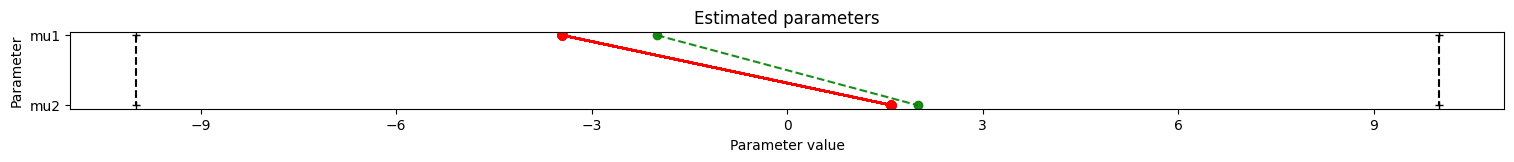
for m in models.values():
    m["results"] = optimize.minimize(
        problem=m["problem"],
        n_starts=100,
    )

    if "true_params" in m.keys():
        visualize.parameters(
            results=m["results"],
            reference={
                "x": m["true_params"],
                "fval": m["problem"].objective(m["true_params"]),
            },
        )
    else:
        visualize.parameters(m["results"])

CPU times: user 1.01 s, sys: 1.15 ms, total: 1.01 s
Wall time: 590 ms

../_images/example_model_evidence_and_bayes_factors_10_1.png

../_images/example_model_evidence_and_bayes_factors_10_2.png

1. Bayesian Information Criterion (BIC)

The BIC is a simple and widely-used approximation to the marginal likelihood. It is computed as:

\[\operatorname{BIC} = k \ln(n) - 2 \ln(\hat{L})\]

where \(k\) is the number of parameters, \(n\) is the number of data points, and \(\hat{L}\) is the maximum likelihood estimate. \(-\frac12 \operatorname{BIC}\) approximates the marginal likelihood under the assumption that the prior is non-informative and the sample size is large.

BIC is easy to compute and converges to the marginal likelihood, but it may not capture the full complexity of model selection, especially for complex models or significant prior information as the prior is completely ignored.

[7]:

for m in models.values():
    m["BIC"] = len(m["problem"].x_free_indices) * np.log(n_obs) + 2 * m[
        "neg_log_likelihood"
    ](m["results"].optimize_result.x[0])
    print(
        m["name"], "BIC marginal likelihood approximation:", -1 / 2 * m["BIC"]
    )

True-Model BIC marginal likelihood approximation: -21.714716595687893
Alternative-Model BIC marginal likelihood approximation: -28.356215203233447

2. Laplace Approximation

The Laplace approximation estimates the marginal likelihood by approximating the posterior distribution as a Gaussian centered at the maximum a posteriori (MAP) estimate \(\hat{\theta}\) using the Hessian of the posterior distribution. The marginal likelihood is then approximated as:

\[P(\mathcal{D} \mid \mathcal{M}) \approx (2\pi)^{k/2} \left| \Sigma \right|^{1/2} P(\mathcal{D} \mid \hat{\theta}, \mathcal{M}) P(\hat{\theta} \mid \mathcal{M})\]

where \(\Sigma\) is the covariance matrix of the posterior distribution (unnormalized, so likelihood \(\times\) prior).

The Laplace approximation is accurate if the posterior is unimodal and roughly Gaussian.

[8]:

%%time
for m in models.values():
    laplace_evidences = []
    for x in m["results"].optimize_result.x:
        log_evidence = sample.evidence.laplace_approximation_log_evidence(
            m["problem"], x
        )
        laplace_evidences.append(log_evidence)

        m["laplace_evidences"] = np.array(laplace_evidences)
    print(m["name"], f"laplace approximation: {m['laplace_evidences'][0]}")

True-Model laplace approximation: -21.42916318626999
Alternative-Model laplace approximation: -27.833962017301445
CPU times: user 74.5 ms, sys: 2.15 ms, total: 76.7 ms
Wall time: 73.7 ms

3. Sampling-Based Methods

Sampling-based methods, such as Markov Chain Monte Carlo (MCMC) or nested sampling, do not make assumptions about the shape of the posterior and can provide more accurate estimates of the marginal likelihood. However, they can be computationally very intensive.

Arithmetic Mean Estimator

The arithmetic mean estimator also uses samples from the prior evaluated at the likelihood function to approximate the marginal likelihood:

\[P(\mathcal{D} \mid \mathcal{M}) \approx \frac{1}{N} \sum_{i=1}^N P(\mathcal{D} \mid \theta_i, \mathcal{M})\]

The arithmetic mean estimator requires a large number of samples and is very inefficient. It approximates the marginal likelihood from below.

[9]:

%%time
for m in models.values():
    prior_sample = np.random.multivariate_normal(
        mean=m["prior_mean"], cov=m["prior_cov"], size=1000
    )
    log_likelihoods = np.array(
        [-m["neg_log_likelihood"](x) for x in prior_sample]
    )
    m["arithmetic_log_evidence"] = logsumexp(log_likelihoods) - np.log(
        log_likelihoods.size
    )

    print(m["name"], f"arithmetic mean: {m['arithmetic_log_evidence']}")

True-Model arithmetic mean: -21.49555889068519
Alternative-Model arithmetic mean: -27.820889217930947
CPU times: user 177 ms, sys: 13.3 ms, total: 190 ms
Wall time: 177 ms

Harmonic Mean

The harmonic mean estimator uses posterior samples to estimate the marginal likelihood:

\[P(\mathcal{D} \mid \mathcal{M}) \approx \left( \frac{1}{N} \sum_{i=1}^N \frac{1}{P(\mathcal{D} \mid \theta_i, \mathcal{M})} \right)^{-1}\]

where \(\theta_i\) are samples from the posterior distribution.

The harmonic mean estimator approximates the evidence from above since it tends to ignore low likelihood regions, such as those comprising the prior, leading to overestimates of the marginal likelihoods, even when asymptotically unbiased. Moreover, the estimator can have a high variance due to evaluating the likelihood at low probability regions and inverting it. Hence, it can be very unstable and even fail catastrophically. A more stable version, the stabilized harmonic mean, also uses samples from the prior (see Newton and Raftery (1994)). However, there are more efficient methods available.

A reliable sampling method is bridge sampling (see “A Tutorial on Bridge Sampling” by Gronau et al. (2017) for a nice introduction). It uses samples from a proposal and the posterior to estimate the marginal likelihood. The proposal distribution should be chosen to have a high overlap with the posterior (we construct it from half of the posterior samples by fitting a Gaussian distribution with the same mean and covariance). This method is more stable than the harmonic mean estimator. However, its accuracy may depend on the choice of the proposal distribution.

A different approach, the learnt harmonic mean estimator, was proposed by McEwen et al. (2021). The estimator solves the large variance problem by interpreting the harmonic mean estimator as importance sampling and introducing a new target distribution, which is learned from the posterior samples. The method can be applied just using samples from the posterior and is implemented in the software package accompanying the paper.

[10]:

%%time
for m in models.values():
    results = sample.sample(
        problem=m["problem"],
        n_samples=1000,
        result=m["results"],
    )
    # compute harmonic mean
    m["harmonic_log_evidence"] = sample.evidence.harmonic_mean_log_evidence(
        results
    )
    print(m["name"], f"harmonic mean: {m['harmonic_log_evidence']}")

Elapsed time: 0.4530983640000006
Geweke burn-in index: 150

True-Model harmonic mean: -20.738001230737744

Elapsed time: 0.39166042300000115
Geweke burn-in index: 250

Alternative-Model harmonic mean: -27.763614820049852
CPU times: user 821 ms, sys: 55.9 ms, total: 877 ms
Wall time: 828 ms

[11]:

%%time
for m in models.values():
    results = sample.sample(
        problem=m["problem"],
        n_samples=800,
        result=m["results"],
    )
    # compute stabilized harmonic mean
    prior_samples = np.random.multivariate_normal(
        mean=m["prior_mean"], cov=m["prior_cov"], size=200
    )
    m["harmonic_stabilized_log_evidence"] = (
        sample.evidence.harmonic_mean_log_evidence(
            result=results,
            prior_samples=prior_samples,
            neg_log_likelihood_fun=m["neg_log_likelihood"],
        )
    )
    print(
        m["name"],
        f"stabilized harmonic mean: {m['harmonic_stabilized_log_evidence']}",
    )

Elapsed time: 0.3607919519999996
Geweke burn-in index: 0

True-Model stabilized harmonic mean: -21.296702862377

Elapsed time: 0.32489940299999986
Geweke burn-in index: 360

Alternative-Model stabilized harmonic mean: -27.829395367307914
CPU times: user 764 ms, sys: 42.7 ms, total: 806 ms
Wall time: 762 ms

[12]:

%%time
for m in models.values():
    results = sample.sample(
        problem=m["problem"],
        n_samples=1000,
        result=m["results"],
    )
    m["bridge_log_evidence"] = sample.evidence.bridge_sampling_log_evidence(
        results
    )
    print(m["name"], f"bridge sampling: {m['bridge_log_evidence']}")

Elapsed time: 0.4115685029999998
Geweke burn-in index: 0
Elapsed time: 0.4475328590000007
Geweke burn-in index: 200

True-Model bridge sampling: -21.535585296744202
Alternative-Model bridge sampling: -27.821505512893612
CPU times: user 1.1 s, sys: 45.8 ms, total: 1.14 s
Wall time: 1.09 s

Nested Sampling

Nested sampling is specifically designed for estimating marginal likelihoods. The static nested sampler is optimized for evidence computation and provides accurate estimates but may give less accurate posterior samples unless dynamic nested sampling is used.

Dynamic nested sampling can improve the accuracy of posterior samples. The package dynesty offers a lot of hyperparameters to tune accuracy and efficiency of computing samples from the posterior vs. estimating the marginal likelihood.

[13]:

%%time
for m in models.values():
    # define prior transformation needed for nested sampling
    def prior_transform(u, m=m):
        """Transform prior sample from unit cube to normal prior."""
        t = stats.norm.ppf(u)  # convert to standard normal
        c_sqrt = np.linalg.cholesky(m["prior_cov"])  # Cholesky decomposition
        u_new = np.dot(c_sqrt, t)  # correlate with appropriate covariance
        u_new += m["prior_mean"]  # add mean
        return u_new

    # initialize nested sampler
    nested_sampler = sample.DynestySampler(
        # sampler_args={'nlive': 250},
        run_args={"maxcall": 1000},
        dynamic=False,  # static nested sampler is optimized for evidence computation
        prior_transform=prior_transform,
    )

    # run nested sampling
    result_dynesty_sample = sample.sample(
        problem=m["problem"], n_samples=None, sampler=nested_sampler
    )

    # extract log evidence
    m["nested_log_evidence"] = nested_sampler.sampler.results.logz[-1]
    print(m["name"], f"nested sampling: {m['nested_log_evidence']}")

Elapsed time: 0.5902764099999995

True-Model nested sampling: -21.509681849053795

Elapsed time: 0.5590382319999989

Alternative-Model nested sampling: -27.84221223401817
CPU times: user 1.44 s, sys: 3.53 ms, total: 1.44 s
Wall time: 1.44 s

Thermodynamic Integration and Steppingstone Sampling

These methods are based on the power posterior, where the posterior is raised to a power \(t\) and integrated over \(t\):

\[P(\mathcal{D} \mid \mathcal{M}) = \int_0^1 \frac1{Z_t} P(\mathcal{D} \mid \theta, \mathcal{M})^t P(\theta \mid \mathcal{M}) \, dt\]

Parallel tempering is a sampling algorithm that improves accuracy for multimodal posteriors by sampling from different temperatures simultaneously and exchanging samples between parallel chains. It can be used to sample from all power posteriors simultaneously allowing for thermodynamic integration and steppingstone sampling (Annis et al., 2019). These methods can be seen as path sampling methods, hence related to bridge sampling.

These methods can be more accurate for complex posteriors but are computationally intensive. Thermodynamic integration (TI) relies on integrating the integral over the temperature \(t\), while steppingstone sampling approximates the integral with a sum over a finite number of temperatures using an importance sampling estimator. Accuracy can be improved by using more temperatures. Errors in the estimator might come from the MCMC sampler in both cases and from numerical integration when applying TI. Steppingstone sampling can be a biased estimator for a small number of temperatures (Annis et al., 2019).

[14]:

%%time
for m in models.values():
    # initialize parallel tempering sampler
    ti_sampler = sample.ParallelTemperingSampler(  # not adaptive, since we want fixed temperatures
        internal_sampler=sample.AdaptiveMetropolisSampler(), n_chains=10
    )

    # run mcmc with parallel tempering
    result_ti = sample.sample(
        problem=m["problem"],
        n_samples=1000,
        sampler=ti_sampler,
        result=m["results"],
    )
    # compute log evidence via thermodynamic integration
    m["thermodynamic_log_evidence"] = (
        sample.evidence.parallel_tempering_log_evidence(
            result_ti, use_all_chains=False
        )
    )
    print(
        m["name"],
        f"thermodynamic integration: {m['thermodynamic_log_evidence']}",
    )

    # compute log evidence via steppingstone sampling
    m["steppingstone_log_evidence"] = (
        sample.evidence.parallel_tempering_log_evidence(
            result_ti, method="steppingstone", use_all_chains=False
        )
    )
    print(
        m["name"], f"steppingstone sampling: {m['steppingstone_log_evidence']}"
    )

Initializing betas with "beta decay".
Initializing parallel chains with a combination of the starting point and prior samples with weight: 0.9.
Elapsed time: 4.049366717
Geweke burn-in index: 0
Burn-in index (0) already calculated. Skipping Geweke test.
Initializing betas with "beta decay".
Initializing parallel chains with a combination of the starting point and prior samples with weight: 0.9.

True-Model thermodynamic integration: -21.40321352907031
True-Model steppingstone sampling: -21.368309915773096

Elapsed time: 4.097733373999997
Geweke burn-in index: 200
Burn in index coincides with chain length. The chain seems to not have converged yet.
You may want to use a larger number of samples.
At least 1 chains seem to not have converged yet. You may want to use a larger number of samples.
Burn-in index (200) already calculated. Skipping Geweke test.
Burn in index coincides with chain length. The chain seems to not have converged yet.
You may want to use a larger number of samples.
At least 1 chains seem to not have converged yet. You may want to use a larger number of samples.

Alternative-Model thermodynamic integration: -27.817410329634956
Alternative-Model steppingstone sampling: -27.811608507683513
CPU times: user 8.56 s, sys: 109 ms, total: 8.67 s
Wall time: 8.56 s

Variational Inference

Variational inference approximates the posterior with a simpler distribution and can be faster than sampling methods for large problems. The marginal likelihood can be estimated using similar approaches as before, but the accuracy is limited by the choice of the variational family.

Variational inference optimization is based on the Evidence Lower Bound (ELBO), providing an additional check for the estimator.

[15]:

%%time
for m in models.values():
    # one could define callbacks to check convergence during optimization
    # import pymc as pm
    # cb = [
    #     pm.callbacks.CheckParametersConvergence(
    #         tolerance=1e-3, diff='absolute'),
    #     pm.callbacks.CheckParametersConvergence(
    #         tolerance=1e-3, diff='relative'),
    # ]

    pypesto_variational_result = variational.variational_fit(
        problem=m["problem"],
        method="advi",
        n_iterations=10000,
        n_samples=None,
        result=m["results"],
        # callbacks=cb,
    )

    # negative elbo, this is bound to the evidence (optimization criterion)
    vi_lower_bound = np.max(
        -pypesto_variational_result.variational_result.data.hist
    )

    # compute harmonic mean from posterior samples
    approx_sample = pypesto_variational_result.variational_result.sample(1000)[
        "trace_x"
    ][0]
    neg_log_likelihoods = np.array(
        [m["neg_log_likelihood"](ps) for ps in approx_sample]
    )
    m["vi_harmonic_log_evidences"] = -logsumexp(neg_log_likelihoods) + np.log(
        neg_log_likelihoods.size
    )
    print(
        m["name"],
        f"harmonic mean with variational inference: {m['vi_harmonic_log_evidences']}",
    )
    print("Evidence lower bound:", vi_lower_bound)

    # evidence cannot be smaller than the lower bound
    m["vi_harmonic_log_evidences"] = max(
        m["vi_harmonic_log_evidences"], vi_lower_bound
    )

Finished [100%]: Average Loss = 27.561
Elapsed time: 6.886745308999998

True-Model harmonic mean with variational inference: -23.399955558008887
Evidence lower bound: -24.802029767873737

Finished [100%]: Average Loss = 31.064
Elapsed time: 5.240469904999998

Alternative-Model harmonic mean with variational inference: -29.935578874836665
Evidence lower bound: -28.971941986308654
CPU times: user 12.2 s, sys: 783 ms, total: 13 s
Wall time: 40.9 s

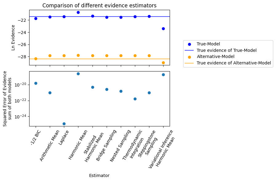
Comparison

[16]:

labels = [
    "-1/2 BIC",
    "Arithmetic Mean",
    "Laplace",
    "Harmonic Mean",
    "Stabilized\nHarmonic Mean",
    "Bridge Sampling",
    "Nested Sampling",
    "Thermodynamic\nIntegration",
    "Steppingstone\nSampling",
    "Variational Inference\nHarmonic Mean",
]

bayes_factors = [
    -1 / 2 * models["mixture_model1"]["BIC"]
    + 1 / 2 * models["mixture_model2"]["BIC"],
    models["mixture_model1"]["arithmetic_log_evidence"]
    - models["mixture_model2"]["arithmetic_log_evidence"],
    models["mixture_model1"]["laplace_evidences"][0]
    - models["mixture_model2"]["laplace_evidences"][0],
    models["mixture_model1"]["harmonic_log_evidence"]
    - models["mixture_model2"]["harmonic_log_evidence"],
    models["mixture_model1"]["harmonic_stabilized_log_evidence"]
    - models["mixture_model2"]["harmonic_stabilized_log_evidence"],
    models["mixture_model1"]["bridge_log_evidence"]
    - models["mixture_model2"]["bridge_log_evidence"],
    models["mixture_model1"]["nested_log_evidence"]
    - models["mixture_model2"]["nested_log_evidence"],
    models["mixture_model1"]["thermodynamic_log_evidence"]
    - models["mixture_model2"]["thermodynamic_log_evidence"],
    models["mixture_model1"]["steppingstone_log_evidence"]
    - models["mixture_model2"]["steppingstone_log_evidence"],
    models["mixture_model1"]["vi_harmonic_log_evidences"]
    - models["mixture_model2"]["vi_harmonic_log_evidences"],
]

true_bf = (
    models["mixture_model1"]["true_log_evidence"]
    - models["mixture_model2"]["true_log_evidence"]
)

[17]:

fig, ax = plt.subplots(2, 1, tight_layout=True, sharex=True, figsize=(6, 6))
colors = ["blue", "orange"]

for i, m in enumerate(models.values()):
    m["log_evidences"] = np.array(
        [
            -1 / 2 * m["BIC"],
            m["arithmetic_log_evidence"],
            m["laplace_evidences"][0],
            m["harmonic_log_evidence"],
            m["harmonic_stabilized_log_evidence"],
            m["bridge_log_evidence"],
            m["nested_log_evidence"],
            m["thermodynamic_log_evidence"],
            m["steppingstone_log_evidence"],
            m["vi_harmonic_log_evidences"],
        ]
    )
    ax[0].scatter(
        x=np.arange(m["log_evidences"].size),
        y=m["log_evidences"],
        color=colors[i],
        label=m["name"],
    )
    ax[0].axhline(
        m["true_log_evidence"],
        color=colors[i],
        alpha=0.75,
        label=f"True evidence of {m['name']}",
    )

    m["error"] = (
        np.exp(m["log_evidences"]) - np.exp(m["true_log_evidence"])
    ) ** 2
mean_error = np.sum(np.array([m["error"] for m in models.values()]), axis=0)
ax[1].scatter(x=np.arange(len(labels)), y=mean_error)

ax[1].set_xlabel("Estimator")
ax[0].set_title("Comparison of different evidence estimators")
ax[0].set_ylabel("Ln Evidence")
ax[1].set_ylabel("Squared Error of Evidence\nsum of both models")
ax[1].set_yscale("log")
ax[1].set_xticks(ticks=np.arange(len(labels)), labels=labels, rotation=60)
fig.legend(ncols=1, loc="center right", bbox_to_anchor=(1.5, 0.7))
plt.show()

../_images/example_model_evidence_and_bayes_factors_30_0.png

[18]:

fig, ax = plt.subplots(1, 1, tight_layout=True, figsize=(6, 5))
ax.axhline(true_bf, linestyle="-", color="r", label="True Bayes Factor")
plt.scatter(
    x=np.arange(len(bayes_factors)), y=bayes_factors, label="Estimates"
)

# add decision thresholds
c = lambda x: np.log(
    np.power(10, x)
)  # usually defined in log10, convert to ln
ax.axhline(
    c(0),
    color="red",
    linestyle="--",
    label='"Not worth more than a bare mention"',
)
ax.axhline(c(0.5), color="orange", linestyle="--", label='"Substantial"')
ax.axhline(c(1), color="yellow", linestyle="--", label='"Strong"')
ax.axhline(c(2), color="green", linestyle="--", label='"Decisive"')

ax.set_ylabel("ln Bayes Factor")
ax.set_xlabel("Estimator")
ax.set_title(
    f"Bayes Factor of {models['mixture_model1']['name']} vs. {models['mixture_model2']['name']}"
)
plt.xticks(ticks=np.arange(len(bayes_factors)), labels=labels, rotation=60)
fig.legend(ncols=1, loc="center right", bbox_to_anchor=(1.5, 0.7))
plt.show()

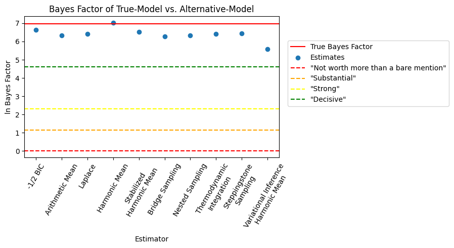
../_images/example_model_evidence_and_bayes_factors_31_0.png

We recommend using either bridge sampling, nested sampling or one of the methods using power posteriors depending on the computational resources available.

Bayes factors and marginal likelihoods are powerful tools for Bayesian model comparison. While there are various methods to compute marginal likelihoods, each has its strengths and weaknesses. Choosing the appropriate method depends on the specific context, the complexity of the models, and the computational resources available.